AI for robotics projects
Computer vision
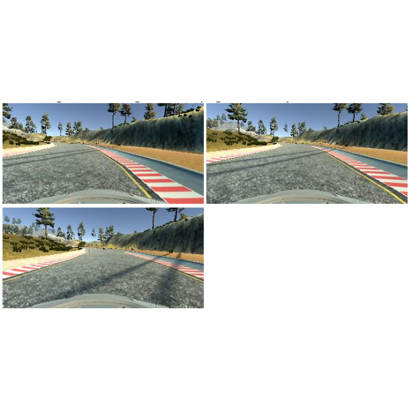
Advanced lane line tracking
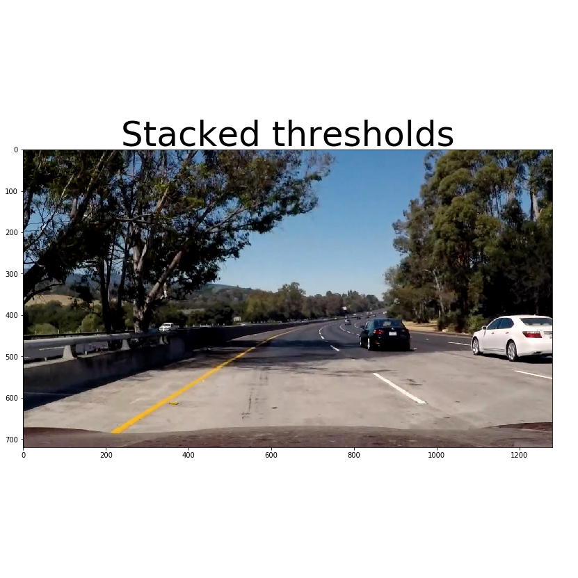
In this project, I developed a software pipeline to identify the lane boundaries of a road in a video. A series of steps are followed to identify the lanes:
- Compute the camera calibration matrix and distortion coefficients given a set of chessboard images.
- Apply a distortion correction to raw images.
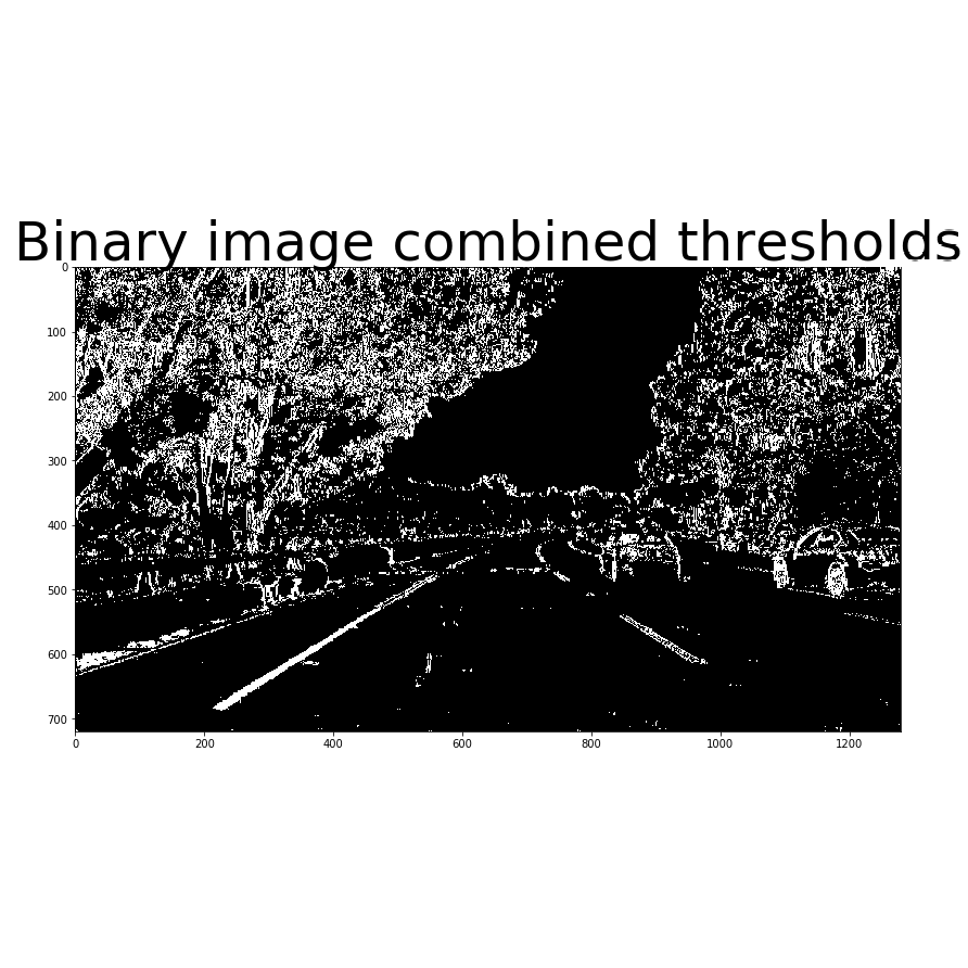
- Use color transforms, gradients, etc., to create a thresholded binary image.
- Apply a perspective transform to rectify binary image ("birds-eye view").
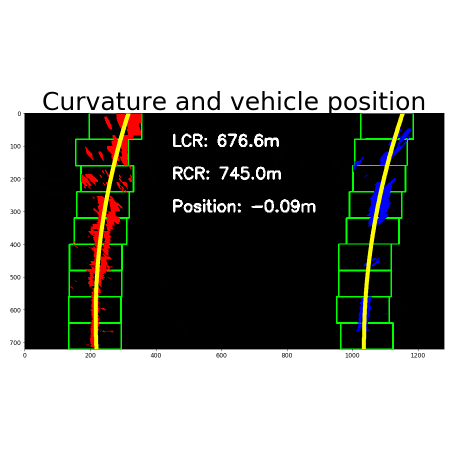
- Detect lane pixels and fit to find the lane boundary.
- Determine the curvature of the lane and vehicle position with respect to center
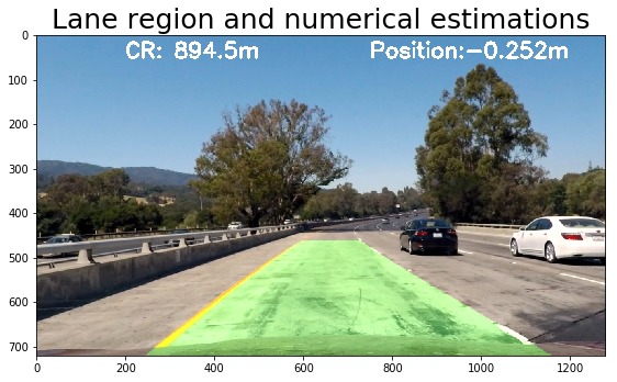
- Warp the detected lane boundaries back onto the original image.
- Output visual display of the lane boundaries and numerical estimation of lane curvature and vehicle position.
The final result is shown in the right hand side image. Steps 3, 4, 5 and 6 are illustrated in the collection of images above.
Source: Advanced lane line tracking.
Traffic signed classifier with CNN
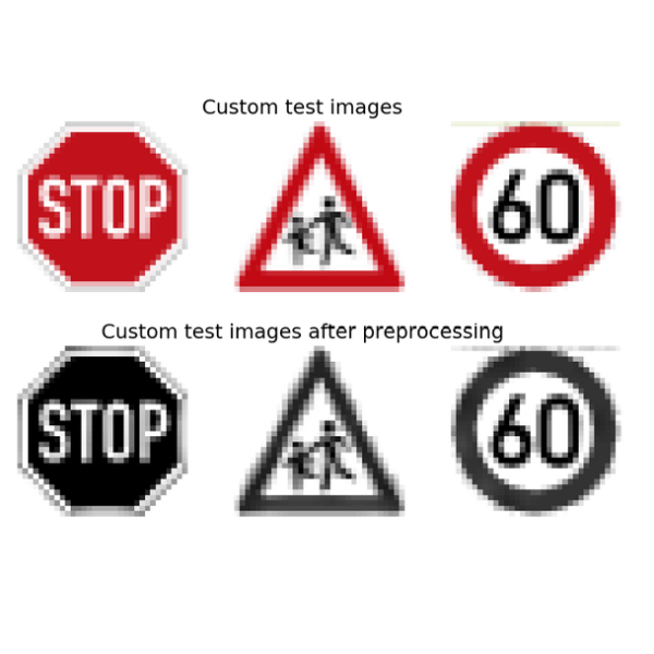
In this project, I used Convolutional Neural Networks to classify traffic signs. An iterative approach was followed to reach a satisfactory solution. The first architecture used was Lenet 5. This network has two convolutional and max-pooling sets. It also lacks dropout implementation and includes three fully connected layers (if we consider the output layer). No data augmentation was implemented and data preprocessing was included in the form of grayscaling and image normalization. The performance achieved during this stage was about 89 percent. After this initial setup, several hyperparameters were modified, the batch size was increased to 128, 256 and 512, the number of epochs was changed between 100 and 200 and I tried with different learning rates. The best ones were values below 0.005. The architecture of the neural network was also modified. The depth of the convolutional layer was also modified, increases in their depth gave better accuracies during training and validation. The initial convolutional layers of the Lenet implementation had a depth of 6 and 16 respectively. This value was increased to 16 and 32, and finally 32 and 64. Additional changes were defined in the output of the fully connected layers: variations went from values for the initial Lenet implementation, 120-84-43, to a bigger number of nodes 800-200-43 and 1000-500-43. After successive increases in the depth of the convolutional layer and output sizes of the fully connected layers, the network gave improvements in validation accuracy between 1% and 3%. The final model results were:
- Training set accuracy of 98.4%.
- Validation set accuracy of 97.2%.
- Test set accuracy of 94.9%.
Source: Traffic sign classifier.
Behavioral cloning
In this project CNNs are used in the process known as imitation learning. An agent (in this case a car) moving in a map (a simulation track) is observed by a neural network and learns to behave like it through imitation. I followed an iterative method to derive the best architecture. Initially started with a simple fully connected layer. The results were not attractive since the vehicle was turning left and right in a constant basis after training and the vehicle motion was far from smooth. Next, I made a transition to a LeNet like network with three convolutional layers and one fully connected layer in addition to the output layer. During model training, the training loss was decreasing while validation loss changed randomly around a fixed value. In simulation testing, the car was able to drive in the straight road but could not complete the curves in several scenarios. The driving style was also far from smooth. The best result was obtained with an architecture that consists of a deep convolutional neural network with a set of five convolutions at the beginning and three fully connected layers in addition to the output layer. The first 3 convolutional layers use a filter of size 5x5, stride of 2x2 and have depths of 24, 32 and 48 respectively. The other 2 convolutional layers use a filter of 3x3, stride of 1x1 and have a depth of 64 (both). To avoid overfitting, validation sets were defined as the 20% of the training set in each epoch. Dropout layers were also used in the convolutional parts of the network. The batch size was set to 32 and Adam optimizer was used to train the model, so the learning rate was not tuned manually. The activation function RELU was used in the convolutional layers. No activation function was used in the fully connected layers.
Source: Behavioral cloning.
Sensor fusion and localization
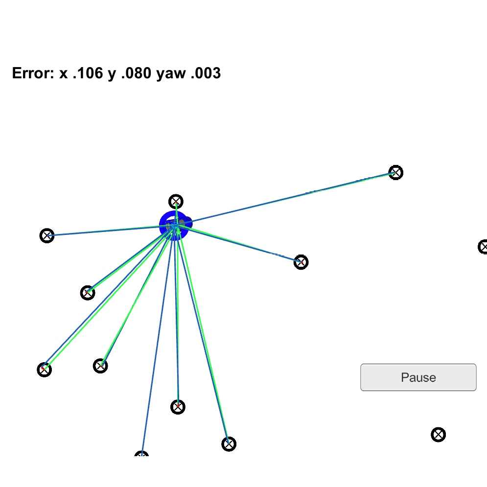
Extended kalman filter
In this project I implemented an enhanced Kalman Filter to estimate the state of a moving object of interest with noisy lidar and radar measurements. The C++ code creates a server with uWebSockets and connects to a client simulator built on the Unity engine. The simulator shows the moving object, laser/radar/estimation data (as red dots, blue circles and green triangles respectively) and RMSE data for position and velocity values in the x and y axis.
Source: Extended kalman filter.
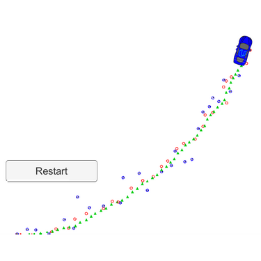
Particle filter
In this project a robot has been kidnapped and transported to a new location. Luckily it has a map of this location, a (noisy) GPS estimate of its initial location, and lots of (noisy) sensor and control data. A two dimensional particle filter implemented in C++ is used to localize the robot from this data. The filter works in the context of a set of landmark data from a map and some initial localization information (similar to what a GPS would provide). At each time step the filter receives observation and control data. This data is then used to perform a set of steps: initilization, prediction, update and resampling.
Source: Particle filter.
Path planning
The path planning algorithm implemented in this project allows the control of an autonomous vehicle in a high-speed highway by enabling behavior selection and trajectory generation features. A class was created containing the main properties (current lane, changing lane status, too_close, too_close_left and too_close_right) and methods required to reach a set of requirements that must be met, for instance:
- The car drives according to a speed limit of 50 miles per hour.
- Max acceleration and jerk don't exceed 10 m/s2 and 10 m/s3 respectively.
- The car doesn't have collisions.
- The car stays in its lane, except for the time when it is changing lanes.
- The car is able to change lanes.
- The car is able to drive in simulation at least 4.32 Miles without incident, meaning any of the previous conditions are satisfied.
Source: Path planning.
PID Controller
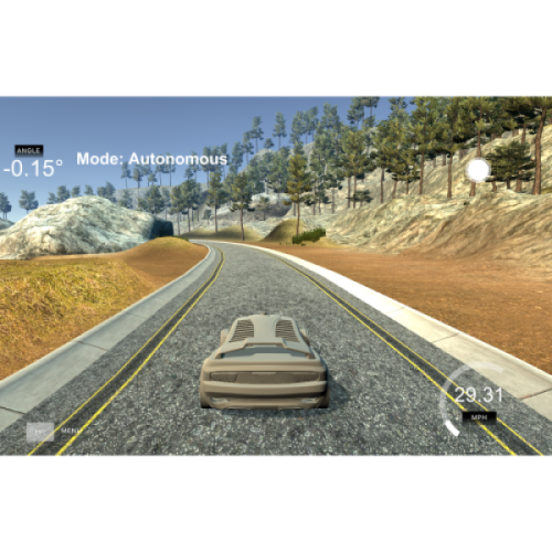
The PID controller, which stands for proportional, integral and differential, is a linear controller designed to stabilize a dynamic linear system in time around an offset value. It is one the most practical and widely used controllers in the industry and I have personally designed one in the past to control a magnetic levitation system, as shown here. One of the most attractive features of the PID controller is that it is quite easy to understand it. It is described by basic Calculus and each term in its mathematical definition tells us what does to the control signal. In this project I described and implemented each term of the controller. In the implementation, the error is the difference between the offset or desired value, and the actual output of the system: (1) error(t) = offset - output(t). dt is the time step or sampling time. The output(t) is the angle in time, which changes in a range from -25 degrees to 25 degrees. Finally, the controller is used in simulation to define the steering angle (output) of the autonomous car. This is considered the final step in a typical pipeline of an autonomous agent software once perception and planning have been completed.
Source: PID controller.
Self driving car pipeline
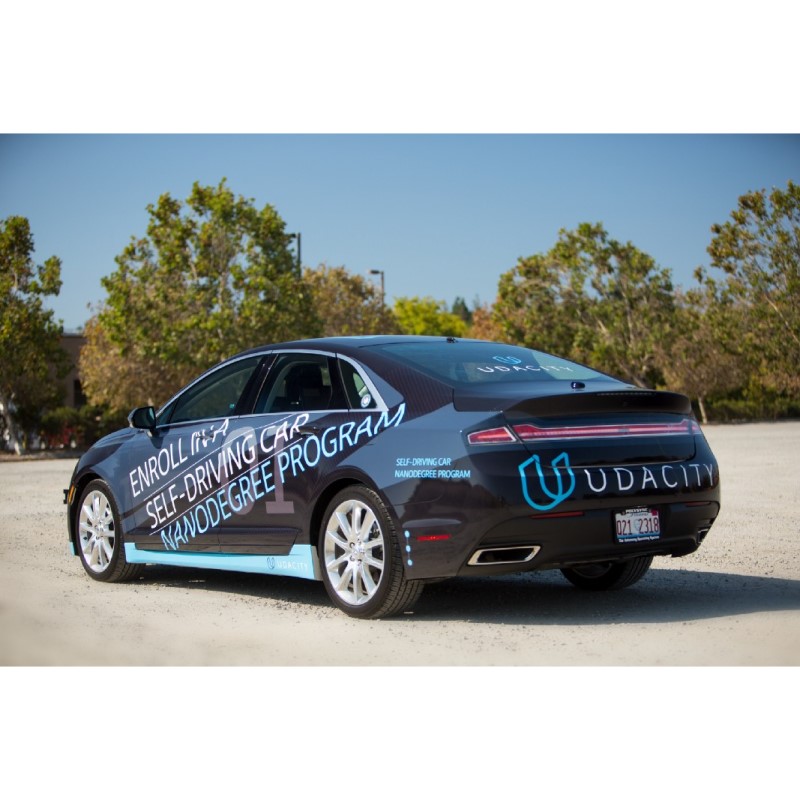
Summary in progress. In the mean time you can explore the Github source.
Source: Self driving car architecture.